A group grid of points (or virtual sensors) are created by an initial model estimate of the conditions at the surface (and above) and that virtual sensor is then nudged by the observations around it to the more accurate value.
 Why Virtual Sensors Could Save California's At-Risk Almond Yields

Caleb Midgley | iteris
To say that the Golden State can lay claim to the title of king of almonds might be an understatement. In 2017, California accounted for nearly 80% of the world’s almond production, a crown jewel in the already impressively productive central valley of the state. But just as it is never wise to have all your financial assets vulnerable to a singular threat, growers, too, must do whatever they can to mitigate risks to their crops. Some things, however, are simply beyond the control of even the best farm management practices, so when a natural event threatens the emerging almond crop in central California, it’s bound to make headlines.
In fact, a perfect example occurred recently. From the morning of February 20, an upper-level trough remained almost stationary across the western US throughout the week, with waves of unseasonably cold air settling into the region, the worst of which occurred on the mornings of February 20 and 24. In the wake of the migrating disturbances moving through the trough, surface high pressure settled in on those two particular mornings, resulting in dry air, light winds and stable conditions. As most almond growers will tell you, these conditions all but guarantee freezing temperatures at a truly inopportune time in the almond growth cycle.
Freezing in February
Why is February 20 such a bad time for a freeze event? Because most varieties were already at 40% or greater bloom during this freeze event, according to the Blue Diamond grower reports. It’s generally understood that nut damage can begin with as little as 30 minutes of exposure to temperatures of 29° F or less during the full bloom and nut stages. On the extreme end of the scale, one of the California Irrigation Management Service (CIMIS) stations near Oakdale dropped as low as 19° F on the morning of February 20, indicating how significant a threat this day posed.
With conditions like this, forward-looking growers cleverly ran sprinklers to combat the effects of the cold temperatures (fun fact: when water freezes it releases heat, raising the temperature of the orchard floor). Others will have used wind machines or even flown helicopters over threatened orchards. Given the labor and time involved with these activities, an orchard-specific temperature data source leading up to the event is essential for properly executing the right activities at the right time and location.
Gaps in the Data
On a 40-acre almond plot, a 10% reduction of almond yield could amount to as much as a $16k loss. With such sizeable losses in revenue, almond growers especially cannot afford to risk damage to their valuable crop. So in the case of February 20, what were their options? For those who had access to localized weather station data alerting them to run their sprinklers, they were probably able to mitigate the damage. But how about those who maybe didn’t have a weather station onsite and relied on publicly available sources?
Figure 1 shows the various publicly available surface weather stations in central California centered near Fresno:
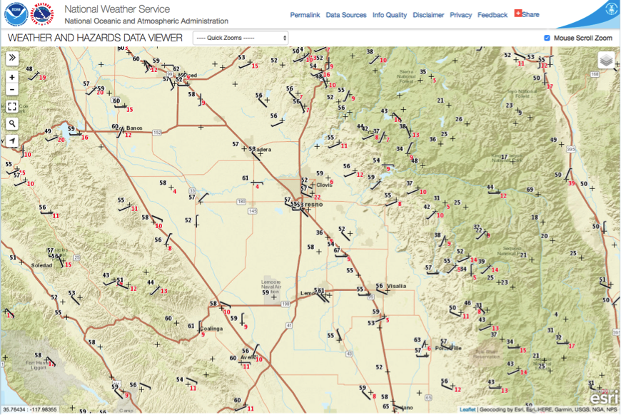
Figure 1 (courtesy of https://www.wrh.noaa.gov/)
Each of the arrows indicates a location where surface temperature is being recorded. However, if you consider the size of an almond orchard, you can see where large distances might exist between a grower’s orchard and a surface observation in the central valley. Other sites, such as the CIMIS weather network, exist that are not shown here, but that does not guarantee the existence of a “close-by” observation. There is also the issue of whether any distant weather station is even representative of your location since terrain features and other factors may mitigate the usefulness of such data. So, what can you do if you would like current conditions and a short-term forecast for one of these gapped regions?
One solution would be to install your own weather station while searching out a weather forecast for that location. Surface weather stations have come very far in instrumentation improvements over the years, but they still cannot forecast weather, nor will they as they are observing systems, not forecast systems. To get the whole picture, you will need to combine observed and forecast data with the assumption that it is all representative of your location. So, there is work and cost here to make this an effective solution, but it is one approach.
Filling in the Holes: Virtual Sensors
Another approach could be the use of a virtual sensor network that has both a historical record and a forecast component. Now at this point some might roll their eyes at the mention of another “virtual” gadget. However, you may already depend on virtual sensors every day. For instance, have you ever depended on a weather forecast from the National Weather Service? Well, these skilled forecasters use model forecast data every day which has to start from somewhere. You may say, “Sure, but the starting point of any forecast has got to be the current conditions coming from a weather station” and you would be somewhat right. However, what about those data holes that we pointed out previously in Figure 1? How do you even begin to make a forecast for those locations given that they do not have any starting point for data if it is indeed observations? The answer to this question can get fairly complex, so we will use a very basic example that is derived from a very old technique.
Let’s say you have some weather observation near a point of interest, but far enough away that you feel a more accurate assessment is needed that takes into account all the available information in the area. One way you can do this is look at the nearest observations and weight the effect of each observation according to the distance to your point of interest. And let’s also say you know the errors associated with those observations. After all, even physical sensors have errors, as they actually depend on physical models themselves that may not always be completely accurate for a given situation. So, if you know the distance of these observations to the point of interest, and you know their errors, you can come up with some sort of “combined” value, with more weight being given to those that are closer and less prone to error. This combined value is your virtual sensor.
Now, in practice, a group grid of points (or virtual sensors) are created by an initial model estimate of the conditions at the surface (and above) and that virtual sensor is then nudged by the observations around it to the more accurate value. Figure 2 gives an example of this initial model estimate with the surrounding observations and their errors.
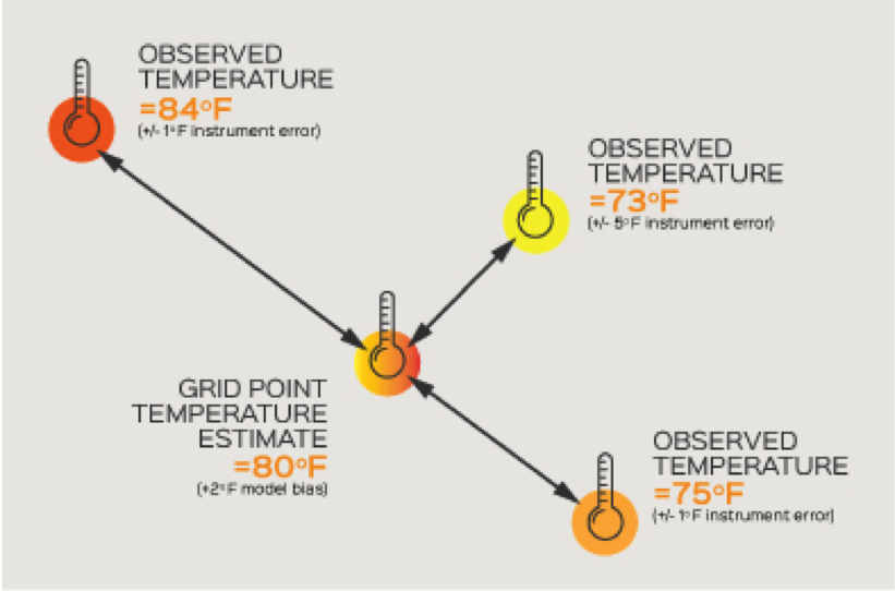
Figure 2
Things are started this way because the model can give you a good initial snapshot of the atmosphere that takes into account all effects and observations. Examples of these other factors include forcing from terrain differences and unique data sources such as upper air observations, to name a few. Then, it’s just a matter of correcting it towards what has been observed. Figure 3 provides the final state of the virtual sensor, denoted as “Grid Point Temperature Estimate”, after taking all these factors into account.
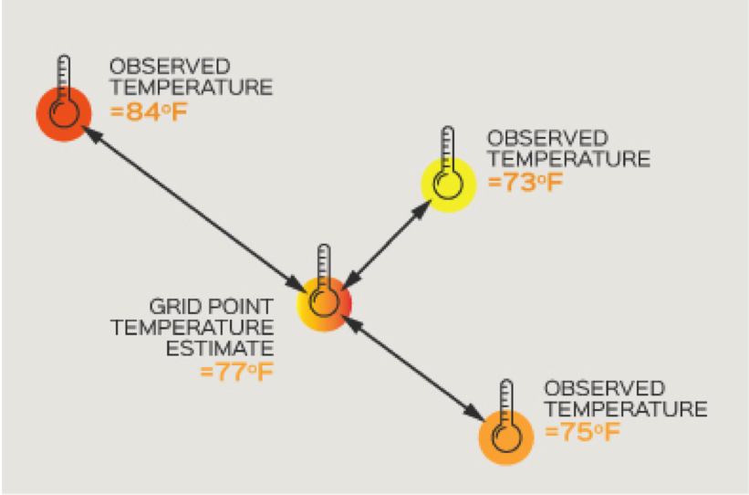
Figure 3
Now, this is a very simple example and it certainly does not contain all the details that are involved with the construction of historical analysis fields. In reality, you would ingest copious amounts of observational data and perform advanced data assimilation techniques to nudge the grid points towards a realistic, observationally influenced value at every point in the analysis, taking into account multiple error and bias sources. The final solution at each grid point is your virtual sensor. We use the generic term sensor because this approach does not only apply to supplementing weather station sensor suites, but even other types of sensors, such as soil moisture sensing hardware. An example of such a surface weather virtual sensor grid can be seen in Figure 4. The circles represent virtual sensor locations while the triangles are METAR locations:
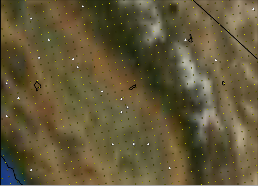
Figure 4
Virtual Sensors Applied
So, this is all well and good as a scientific exercise, but what application could this have in the real world? Well, let’s turn back to our almond freezing event in February 2018. Thanks to the existence of an observational network that is not currently ingested into our virtual sensor generation platform, we do have some examples of virtual sensor performance. This network, the CIMIS from the California Department of Water Resources (www.cimis.water.ca.gov), provides a publically available source of surface weather station data throughout the state.
A few caveats: First, our virtual sensors estimate temperature at 2 meters, while the CIMIS stations have sensors at 1.5 meters. Not a huge difference for most conditions, but different nonetheless. Second, we are providing temperature values for a given moment, whereas the sensors are providing an average value for the hour. Should there be significant changes within the hour to temperature, this can create discrepancies.
With this in mind, let’s look at the comparisons. Figure 5 shows hourly temperature comparisons between a particular CIMIS station and a virtual weather sensor at that same location for three cases: Madera, Parlier and Porterville. The virtual weather sensor data was generated from the ClearAg WeatherPlot application. With 30 years of data archived, as well as nine days of forecast information for any location in the globe, the WeatherPlot tool can provide virtual sensor data on demand for both forward-looking and past event analysis. In this case, WeatherPlot was queried at the location of the CIMIS stations for February 20, with the data subsequently downloaded and plotted in a spreadsheet application. The red-dashed horizontal line is your critical temperature of 29° F. Periods of 30 minutes or more below this line indicate the potential for damage to the almond crop at that location.
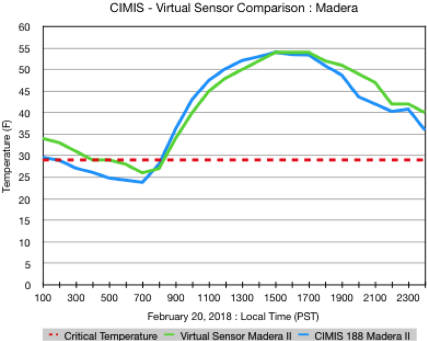
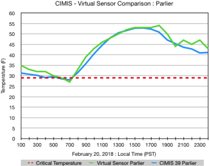
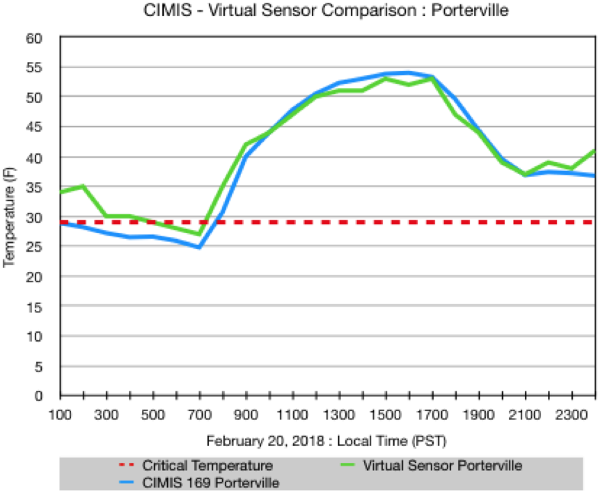
Figure 5. WeatherPlot derived virtual sensors at 3 different locations
As you can see, in all locations the virtual sensors follow closely with the CIMIS plots and also handle the damage level time periods fairly well. Madera and Porterville virtual sensor data tended to be a bit warmer in the overnight hours, but the trend and the critical levels are represented well. Great stuff, but in the end, does this help in solving problems for those in the almond production industry? Well, if you happen to be that individual who is far away from a weather station as we noted previously, virtual sensor temperature data trends might help in making decisions on when and where to turn on sprinklers and/or run wind machines or fly helicopters. Apart from the frost scenario, temperature data such as that above can be used in various growing degree-based models for key management markers such as pest emergence and/or hull split.
What about other uses of virtual sensor data? Given that virtual sensors can provide air temperature, relative humidity, wind speed, solar radiation, precipitation amounts, soil temperature and soil moisture, it makes sense that irrigation management decisions could be a natural application of such data.
Figure 6 is an example of applying virtual sensor data to the problem of assessing soil moisture and irrigation management needs. In this figure, you can see a comparison plot between a cosmic ray neutron probe (yes, they exist, and no I do not have one) and output from a land surface model (denoted “ClearAg”) that utilized virtual sensor information and irrigation activity data:
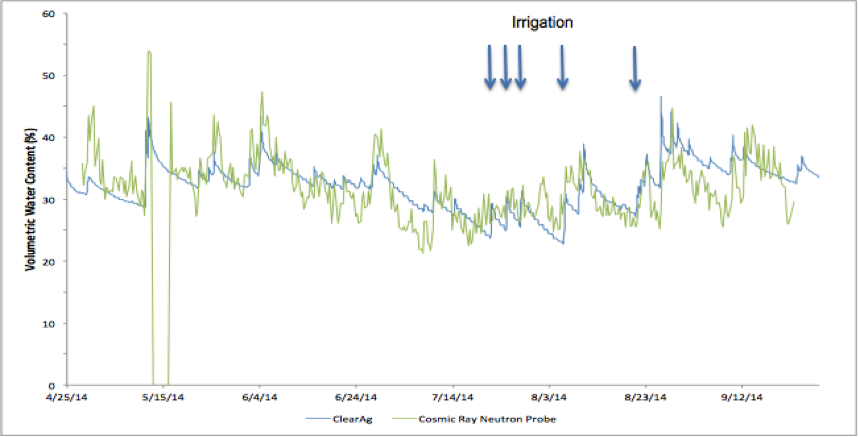
Figure 6
So as you can see, if you are without physical sensor information at your orchard, all is not lost when it comes to understanding the past and future environmental effects on your crop. That isn’t to say physical sensors are not useful. On the contrary, we can’t create a useful virtual sensor solution without the benefit of a solid observational network of physical sensors that inform gridded model data sets. Additionally, locations with significant terrain differences nearby may benefit from localized weather observations due to the highly variable conditions in time and space that are possible at such locations. However, the approach of choosing one solution over the other is really a false choice. If you have a sensor in your orchard, great! Conversely, if you do not, there are solutions out there that do not require extensive internet searches to identify nearby weather station data sets or investing a lot of money to maintain one at your site. And isn’t that the best place to be? A consumer by choice and not relegated to a one-size-fits-all solution? We think so. Happy sensing!
About Caleb Midgley
Caleb Midgley is Scientific Software Project Manager at Iteris, a global leader in applied informatics for transportation and agriculture.
The content & opinions in this article are the author’s and do not necessarily represent the views of AgriTechTomorrow
Comments (0)
This post does not have any comments. Be the first to leave a comment below.
Featured Product
